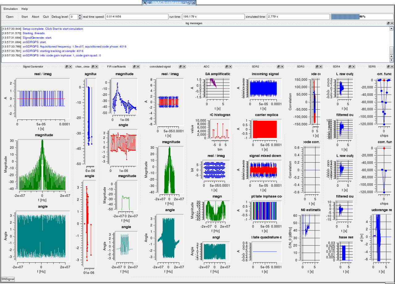
This example explains the simulation with the channel impulse response (CIR) file which was generated in Example05.
The same signal is defined for both signal generation and tracking.
The complete SNACS configuration file for this example is given below. The noise module is commented out to see the isolated multipath effect caused by the channel.
You can use the MATLAB script plot_snacs_results_example06.m to plot the results:
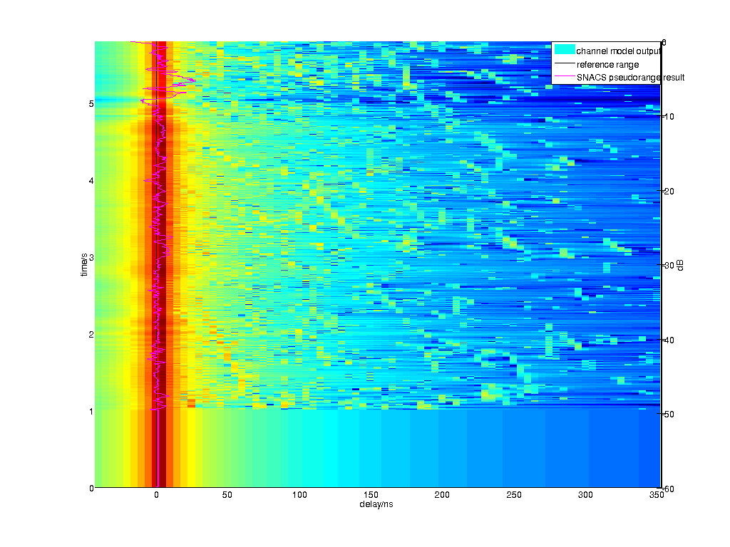
The MATLAB script plot_snacs_results_with_cir_file_example06.m displays the CIR, the reference ranges and the SNACS pseudorange result into one plot:
1 %%%%%%%%%%%%%%%%%%%%%%%%%%%%%%%%%%%%%%%%%%%%%%%%%%%%%%%%%%%%%%%%%%%%%%%%%%
3 % Supporting script
for
5 % SNACS - The Satellite Navigation Radio Channel Simulator
7 % plot_snacs_results_example06.m
9 % MATLAB script for displaying results of SNACS Example 02 simulation.
11 % Copyright (C) 2010 F. M. Schubert
13 % This program is free software: you can redistribute it and/or modify
14 % it under the terms of the GNU General Public License as published by
15 % the Free Software Foundation, either version 3 of the License, or
16 % (at your option) any later version.
18 % This program is distributed in the hope that it will be useful,
19 % but WITHOUT ANY WARRANTY; without even the implied warranty of
20 % MERCHANTABILITY or FITNESS FOR A PARTICULAR PURPOSE. See the
21 % GNU General Public License
for more details.
23 % You should have received a copy of the GNU General Public License
24 % along with
this program. If not, see <http:
26 %%%%%%%%%%%%%%%%%%%%%%%%%%%%%%%%%%%%%%%%%%%%%%%%%%%%%%%%%%%%%%%%%%%%%%%%%%
32 addpath(
'../helper_functions');
34 cir_file =
'../example_05/snacs-cir-file_DLRLMS_example-05.h5';
35 snacs_result_file =
'/tmp/snacs-result_example06/result.h5';
37 %% set interpolation parameters:
38 interp.skip_amount = 1; % interpolate only every interp.skip_amount-th CIR.
39 interp.bandwidth = 100e6; % in Hz, defines the interpolation resolution
40 interp.max_length = 400e-9; % in s, the length up to which the cirs will be plotted
41 interp.move_to_delay0 =
false;
42 interp.add_delay_offset = 43e-9; % in s,
this is added to the reference range
for better visualization
44 %% set plotting parameters:
45 plotting.length = 5.8; % s, total length of plot
46 plotting.range_dB = [-60, 0]; % 2x in dB, plots values within
this dB range
47 plotting.show_title = 0; % print title into figure?
48 plotting.line_width = 3;
49 plotting.font_size = 14;
50 plotting.save = 1; % save plot?
51 plotting.width = 1024;
52 plotting.height = 768;
53 plotting.save_name = [ '../../documentation/doxygen-sources/graphic/snacs-result-and-cir_example06.png' ];
55 %% plot the CIR first and
get the reference ranges:
56 [ reference_ranges, delay_axis, sim_params ] = plot_snacs_cir_file(cir_file, interp, plotting);
58 %%
get the pseudoranges:
59 pseudoranges = hdf5read(snacs_result_file,
'/snSDRGPS/output/pr');
61 %% plot the reference range:
63 % calculate correct axis values first
64 ref_y_axis = 0:1/sim_params.cir_rate:plotting.length-1/sim_params.cir_rate;
65 % trim the number of reference_ranges to the plot length:
66 reference_ranges = reference_ranges(1:numel(ref_y_axis));
67 % reference_ranges are in m. transform to seconds:
68 reference_ranges = reference_ranges / sim_params.c0;
70 plot(reference_ranges/1e-9, ref_y_axis,
'k',
'LineWidth', plotting.line_width);
72 %% plot the pseudorange:
74 % calculate correct axis values first
75 pr_y_axis = 0:1/sim_params.cir_rate:plotting.length-1/sim_params.cir_rate;
76 % trim the number of reference_ranges to the plot length:
77 pseudoranges = pseudoranges(1:numel(ref_y_axis));
78 % reference_ranges are in m. transform to seconds:
79 pseudoranges = pseudoranges / sim_params.c0;
81 plot(pseudoranges/1e-9, pr_y_axis,
'm',
'LineWidth', plotting.line_width);
83 legend(
'channel model output',
'reference range',
'SNACS pseudorange result');
87 save_figure_as_png(plotting.save_name, 1024, 768);
17 sampling_frequency = 40e6;
21 conc_buf_length = 0.001;
22 buffers_per_concbuf = 2;
24 result_directory =
"/tmp/snacs-result_example06";
25 append_date_to_outdir =
false;
28 { Type =
"snSignalGenerate";
34 modulation =
"BPSK(n)";
48 file =
"../../examples/example_05/snacs-cir-file_DLRLMS_example-05.h5";
49 interpolation_type =
"SINC";
50 interpolation_bandwidth = 10.23e6;
54 intermediate_frequency = 15e6;
58 vga_lowest_amplification_dB = -6.0;
59 vga_highest_amplification_dB = 42.5;
62 { Type =
"snSDRStandard";
68 modulation =
"BPSK(n)";
74 intermediate_frequency = 15e6;
75 aquisition_enable =
true;
81 aq_freq_band = 10000.0;
86 tracking_enable =
true;
91 discriminator_type =
"EML";
92 correlation_length = 0.001;
93 early_late_spacing = 1.0;
94 damping_ratio = 0.707;
95 noise_bandwidth = 5.0;
97 corr_func_samples = 13;
98 corr_func_start = -1.5;
99 corr_func_dist = 0.25;
101 write_corr_func =
false;
105 damping_ratio = 0.707;
106 noise_bandwidth = 25.0;
116 UpdateInterval = 500;
118 plot_buffer_length = 0.0001;


 1.8.5
1.8.5